Anticipatory Coordination via Peer-State Prediction Under Communication Delay
We measure how much of the coordination quality lost to communication delay a cheap peer-state predictor buys back, and show that a constant-velocity predictor recovers most of it — with the largest gains exactly where the un-anticipated swarm has already collapsed.
Chris Adams
Arboria Labs, Alpharetta, GA United States
Corresponding Author email: cadams@arborialabs.com
Abstract
A companion study shows that decentralized coordination collapses as communication delay approaches the coordination timescale, and that the collapse is primitive-independent. Here we ask the natural follow-up: if an agent cannot receive fresh peer state, can it anticipate it? We add a decide-on-prediction hook — each agent extrapolates its delayed view of peers forward by the delay horizon and coordinates on the predicted “now,” while the ground-truth state reconciles when the delayed information actually arrives. We evaluate three cheap, deterministic predictors — constant-velocity, a per-agent Kalman filter, and a windowed linear fit — against a no-prediction baseline across a delay sweep on the same rendezvous and consensus tasks. Prediction recovers a large fraction of the delay-lost quality: on consensus at delay , where no-prediction sits at , constant-velocity holds . The ranking is consistent across delays and tasks — constant-velocity linear Kalman none — and the recovery is largest precisely where the un-anticipated swarm has collapsed, i.e. anticipation shifts the collapse boundary outward. We frame the result honestly: the baseline predictors are the result; a learned graph predictor is a stretch direction, not the gate. All numbers regenerate from a committed set of experiment records ( cells, seeds each; NaN).
Keywords
Anticipatory Coordination, Peer-State Prediction, Communication Delay, Consensus, Rendezvous, Multi-Agent Systems
1. Introduction
1.1. Motivation. When communication delay exceeds the coordination timescale, an agent’s picture of its peers is stale, and decentralized coordination collapses over a sharp boundary — the delay cliff (companion paper, Phase Diagram of Decentralized Coordination Under Communication Delay). Stale information, however, is not useless information: if peers move smoothly, an agent can extrapolate the delayed view forward and act on an estimate of the present. This is the anticipation hypothesis — that cheap forward prediction of peer state recovers coordination quality that raw delay destroys.
1.2. Contributions.
- A decide-on-prediction / reconcile-with-truth coordination hook: predict peer state forward by the delay horizon, coordinate on the prediction, reconcile with ground truth as delayed information arrives (§3).
- Head-to-head evaluation of three deterministic predictors — constant-velocity, Kalman, linear — against a no-prediction baseline across delay, on rendezvous and consensus (§4–5).
- The empirical prediction-gain curves: how much quality is recovered, and where the recovery is largest relative to the un-anticipated collapse boundary (§5).
1.3. Outline. §2 relates this to anticipation in networked control. §3 defines the prediction hook and predictors. §4 gives the setup. §5 presents the prediction-gain results. §6 scopes the claim. §7 concludes.
2. Related Work / Background
2.1. Prediction against delay. Compensating for communication or transport delay by predicting remote state is a classical idea. Dead-reckoning with periodic correction underpins distributed interactive simulation (the DIS standard [1]) and networked games; Kalman filtering [2] provides the optimal linear estimator for a constant-velocity motion model; model-predictive control [3] rolls a model forward over a horizon to act ahead of measured state. Our constant-velocity, Kalman, and linear predictors are the standard members of this family.
2.2. What we measure differently. Prior work asks how accurately remote state can be estimated. We instead ask how much coordination quality an estimate recovers on a shared task substrate, measured relative to a known collapse boundary (the companion phase-diagram paper [4]). This reframes prediction from an estimation-error question into a task-outcome question, and lets us say precisely where anticipation matters — at the delays where the un-anticipated swarm has already fallen off the delay cliff.
2.3. Honest gating. We deliberately gate the result on baseline predictors rather than a learned model, so the contribution is a reproducible measurement, not an architecture. A learned graph predictor that anticipates peer intent rather than kinematics is a stretch direction (§6), explicitly not the headline.
3. Method
3.1. Decide-on-prediction, reconcile-with-truth. As in the companion harness, at step each agent observes the true peer snapshot from . With prediction enabled, the agent does not coordinate on that stale snapshot directly: it feeds the delayed view through a predictor to estimate peer state at the present step,
and the coordination primitive acts on . The prediction never mutates ground truth — when the delayed information arrives it reconciles the agent’s record — so anticipation only fills the delay gap for the decision. The extrapolation is scored against the realized state each step for calibration.
3.2. Predictors. All three are cheap, deterministic, and torch-free:
- constant-velocity — ; exact on any constant-velocity trajectory, the minimal anticipatory model;
- Kalman — a per-agent constant-velocity Kalman filter (position + velocity per axis), re-filtered over the history window each step and rolled forward steps;
- linear — a least-squares line fit over the recent window, extrapolated.
The coordination primitive is held fixed (gossip-consensus) so the only variable is the predictor.
4. Experimental Setup
Runs use the same stack and disabled energy/fault modules as the companion paper. The grid is task predictor delay seed cells, with the gossip primitive at ; predictors are and delays are steps (delay is excluded — anticipation only matters under delay). Every point is a mean over seeds; the run produced non-finite values.
5. Results
Fig. 1 is the main result. On consensus, the no-prediction baseline degrades from (delay ) to (delay ) and (delay ). Constant-velocity prediction holds across the same delays — recovering the swarm at delay from to . The ranking is consistent — constant-velocity linear Kalman none — on both tasks, and the gain (predictor minus baseline) is largest at the delays where the un-anticipated swarm has already collapsed. Anticipation therefore shifts the collapse boundary outward rather than merely lifting quality uniformly.
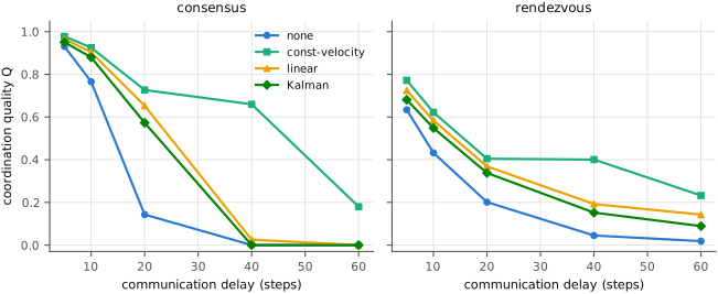
Table 1 gives the per-cell consensus numbers behind Fig. 1. The gain column (const-velocity minus none) is the load-bearing quantity: it is small where the baseline still copes (delay 5–10) and large exactly at the delays where the un-anticipated swarm has collapsed (delay 20–40), which is what “shifting the collapse boundary outward” means.
Table 1. Coordination quality on consensus versus one-way delay (steps), gossip primitive, , mean over 5 seeds. Gain = const-velocity − none. From the committed dcc_p3 records; the linear and Kalman arms fall between these two per the ranking const-velocity linear Kalman none (full arms in Appendix B).
| Predictor | d=5 | d=10 | d=20 | d=40 | d=60 |
|---|---|---|---|---|---|
| none (baseline) | 0.93 | 0.77 | 0.14 | 0.00 | 0.00 |
| const-velocity | 0.98 | 0.93 | 0.73 | 0.66 | 0.18 |
| gain (cv − none) | +0.05 | +0.16 | +0.59 | +0.66 | +0.18 |
That the simplest predictor wins is consistent with the swarm’s dynamics: agents move smoothly under bounded actuation, so a constant-velocity extrapolation is well matched to the horizon, while the Kalman filter’s added variance offers no advantage here and its process/measurement priors cost accuracy at long horizons. An interactive version of the figures (hover for per-point values) is available as a companion artifact.
6. Discussion, Scope, and Limitations
This is a simulation-based algorithmic result in a simplified 3-D kinematic engine. The claim is scoped to the baseline predictors: cheap forward extrapolation recovers most of the delay-lost coordination quality on the studied tasks, with constant-velocity the strongest. A learned graph predictor — trained offline on rollouts to anticipate peer intent rather than kinematics — is a stretch direction and is explicitly not the result here. The prediction gain is measured relative to the companion paper’s collapse boundary and inherits its scope (peer-derived-target tasks; kinematic simulator). Prediction quality is bounded by trajectory smoothness; under sharper maneuvering or adversarial peers the constant-velocity advantage would narrow.
7. Conclusion
Cheap, deterministic peer-state prediction buys back a large fraction of the coordination quality that communication delay destroys, and does so most where it matters — at the delays where the un-anticipated swarm has collapsed. Constant-velocity extrapolation is the strongest of the baselines and the honest headline: anticipation shifts the delay-collapse boundary outward at negligible cost, before any learned model is introduced.
Data and Code Availability
All numbers and figures regenerate from the committed dcc_p3 experiment records (200 cells, 5 seeds each) via Maneuver.Map’s analysis path. The prediction hook (decide-on-prediction / reconcile-with-truth) is in Maneuver.Map’s runner.py; the three predictors are in Gossamer’s prediction/ package (const_velocity, kalman, linear). Each cell writes an experiment.json with a provenance block. The pinned wheel and base-image digests, batch identity, and seed tree are given in Appendix C; the lab’s disclosure policy is at Reproducibility and Data Availability.
References
[1] IEEE Std 1278.1, “Standard for Distributed Interactive Simulation (DIS) — Application Protocols” (dead-reckoning of remote entity state), 2012. [2] Kalman, R. E., “A New Approach to Linear Filtering and Prediction Problems,” Trans. ASME J. Basic Eng., 1960. [3] García, C. E., Prett, D. M., Morari, M., “Model Predictive Control: Theory and Practice — A Survey,” Automatica, 1989. [4] Adams, C., “Phase Diagram of Decentralized Coordination Under Communication Delay,” Arboria Labs, 2026 (companion paper). [5] Olfati-Saber, R., Murray, R. M., “Consensus Problems in Networks of Agents with Switching Topology and Time-Delays,” IEEE Trans. Automatic Control, 2004. [6] Reynolds, C. W., “Flocks, Herds, and Schools: A Distributed Behavioral Model,” SIGGRAPH, 1987.
Appendix / Supplementary Material
Appendix A: Predictors. All three are cheap, deterministic, and free of learned parameters. Given the delayed peer snapshot the agent estimates the present as and coordinates on the estimate; the prediction never mutates ground truth (it reconciles when the delayed information arrives).
- constant-velocity — ; exact on any constant-velocity trajectory, the minimal anticipatory model.
- Kalman — a per-agent constant-velocity Kalman filter (position + velocity per axis), re-filtered over the history window each step and rolled forward steps.
- linear — a least-squares line fit over the recent window (default length 8), extrapolated by steps.
The coordination primitive is held fixed (gossip-consensus) so the only variable is the predictor.
Appendix B: Predictor ranking. Across both tasks and all delays the ordering is constant-velocity linear Kalman none. The linear arm tracks constant-velocity closely because bounded actuation keeps trajectories near-linear over the horizon; Kalman trails because its process/measurement priors add variance that is not repaid on smooth trajectories, and the penalty grows with horizon. The gain over the no-prediction baseline (Table 1) is largest at the delays where the un-anticipated swarm has already collapsed, which is the sense in which anticipation shifts the collapse boundary outward rather than lifting quality uniformly.
Appendix C: Reproducibility checklist.
Canonical batch. Numbers derive from the committed dcc_p3 batch (dcc_p3-20260708T130306-5d8c150d, 200 cells).
The grid. Task predictor delay seed . Tasks rendezvous and consensus; predictors none, const_vel, kalman, linear (history window 8); delays steps — delay 0 is excluded because anticipation only matters under delay. The gossip primitive is held fixed at so the predictor is the only variable, and the remaining parameters match the companion paper (energy_rate=0, fault_prob=0, dt=1, tau_sec=300, steps=1500).
The prediction hook. At each step the runner feeds the agent’s delayed peer view through the predictor, extrapolates it forward by the delay horizon, and lets the coordination primitive act on that estimate. The prediction is scored against the realized state for calibration and never mutates ground truth; actuation always references the agent’s true velocity.
Environment. Gossamer 0.3.1 (wheel SHA256 b28a5335…); Leviathan base image leviathan-base:py-0.2.1 (digest 1ed753f5…); Python 3.10.12 on Linux x86_64 (glibc 2.35). The lockfile hash in provenance.packages.installed_hash is dc55b4a6…, identical to the dcc_p1 environment.
Provenance. Each cell records package versions, the lockfile hash, a hardware fingerprint, and the full seed tree; the git fields are null under the in-process container worker, so the lockfile hash and image digest are the reproducible identity. The run produced 0 non-finite values. On requesting the underlying artifacts, see Reproducibility and Data Availability.
Appendix D: Unified symbols. (coordination quality) and the delayed-coordination substrate follow the companion paper and the shared unified symbols table.
The phase-diagram companion is Phase Diagram of Decentralized Coordination Under Communication Delay.