Energy-Aware Hierarchical Markets: Decentralized Auctions for Autonomous Lunar Construction
We coordinate millimeter-scale micro swarms and macro-scale robotic fleets for lunar ISRU construction using a hierarchical energy-aware market with depot buffering, evaluating against a real OR-Tools MILP planner baseline and adding a queueing-theoretic decoupling result.
Chris Adams
Arboria Labs, Alpharetta, GA United States
Corresponding Author email: cadams@arborialabs.com
Abstract
We study coordinated operations between millimeter-scale micro swarms (regolith processing) and macro-scale robots (haulers, printers) for lunar in-situ resource utilization (ISRU). We propose a hierarchical market-based scheduler with energy-aware auctions (HMA), implemented in Gossamer and executed in Leviathan with energy fields, a range-limited communication model, and OpenMP-parallel physics. Micro swarms locally optimize excavation and compaction; macro fleets allocate hauling tasks via decentralized auctions in which a hauler’s bid is the mass recovered per joule, gated by a state-of-charge sigmoid so that a depleted hauler withdraws from the market rather than stranding itself. We compare against (i) first-come-first-serve (FCFS) and (ii) a MILP central planner built on OR-Tools under a fixed per-replan time budget — a credible centralized comparator, and a deliberately harder test than the greedy baselines this literature usually adopts.
Our central finding is that the market’s advantage is real, large, and confined to scarcity — and that outside scarcity it is a measurable liability. Across 20 seeds per cell, HMA raises printed mass by +33.6% over FCFS when hauling capacity is genuinely scarce (95% CI [+1,979, +7,767] kg; ), with the budgeted central planner close behind at +30.5%. One rung up the capacity ladder the effect is a null (−7.3%, CI [−7,590, +2,395], ). One rung further, when haulers are over-provisioned, the market is significantly worse than the naive baseline — −11.2% printed mass (CI [−10,384, −3,373], ) at +13.6% mobility energy per kilogram. Every claim a market makes must therefore carry a capacity precondition, not merely a capacity caveat: a workload market run on an over-provisioned fleet does not merely fail to help, it costs you throughput.
Two further results are negative, and we report them as such because both refute positions we previously took. First, the depots are saturated in every regime we measured ( in all 180 cells, including the over-provisioned arm), so the M/M/c buffer-decoupling mechanism we introduced in §3.5 does not apply anywhere in this study; what the market actually does — and only under scarcity — is drain a saturated backlog faster at matched arrival rate. Second, and more sharply: the market is not the more predictable scheduler. An earlier version of this paper argued that HMA “degrades gracefully” where the budgeted planner degrades erratically. At 20 seeds that is false in the other direction — HMA’s seed-to-seed standard deviation is 1.5× to 3.4× FCFS’s at every capacity, on every metric, and at the scarce operating point it exceeds the central planner’s too. The market buys throughput under scarcity by increasing variance, and a robustness argument for decentralization is not available from this data.
All results are in raw simulation units; the physical-unit projection of §5.7 is an un-calibrated design target and is not a result. This paper supersedes a 5-seed version whose headline (+29% at hauler capacity 25) does not reproduce; the history, the cause, and what changed are documented in Appendix F rather than quietly restated.
Keywords
Planetary Construction, Market-Based Scheduling, Energy-Aware Auctions, Swarm Robotics, Regolith Processing, Multi-Agent Systems
1. Introduction
1.1. Background and Motivation. Planetary bases require continuous excavation, hauling, and printing under harsh conditions. Micro swarms offer parallelism and adaptability; macro robots provide capacity and reach. Coordinating rates and energy across scales is non-trivial. The gap is robust decentralized scheduling that balances energy, wear, and spatial constraints while preserving emergent efficiencies at micro scale.
1.2. Problem Statement and Research Questions/Hypotheses. We seek to maximize regolith-to-structure throughput while minimizing energy/kg and downtime under failures and variable resources. Our hypotheses are: (H1) Energy-aware auctions increase throughput and reduce idle time versus FCFS; (H2) Buffer depots decouple macro–micro rate mismatches, improving stability.
1.3. Proposed Approach and Contributions. We develop a hierarchical market-based scheduler (HMA) with energy-aware auctions and depot buffering, implemented in Gossamer; Leviathan simulates energy fields, terrain, and queues. The mechanism contributions are the energy-aware auction itself — bids priced as mass recovered per joule, gated by a state-of-charge sigmoid — and a depot ledger held as a PN-counter CRDT so the market remains correct without a consistent global view.
The empirical contribution is a boundary rather than a gain, and we state it that way from the outset because it is the part that is easy to get wrong: measured across 20 seeds per cell against both a naive baseline and a budgeted OR-Tools central planner, the market’s throughput advantage is large under hauling scarcity (+33.6%) and negative when haulers are over-provisioned (−11.2%). We do not claim an energy-per-kilogram gain (it does not survive; §5.3), we do not claim reduced idle time (a flat null; §5.1), and we do not claim robustness or graceful degradation (the market is the least consistent scheduler we tested; §5.5). Nothing here is demonstrated under agent failure: the fault module is disabled in every run so that the scheduler is the only variable.
1.4. Paper Outline. Section 2 reviews related work. Section 3 details HMA. Section 4 describes experiments. Section 5 reports results. Sections 6–8 discuss, limit, and conclude.
2. Related Work / Background
2.1. Market-based task allocation. Allocating tasks to agents by negotiation rather than by decree goes back to the Contract Net protocol [1], in which nodes announce tasks, receive bids, and award contracts — the direct ancestor of the auction in §3.2. The multi-robot community formalized what such mechanisms can and cannot achieve: Gerkey and Matarić [3] give a taxonomy of multi-robot task allocation and, crucially for us, show that the common single-task/single-robot instantaneous-assignment problem is an instance of the optimal assignment problem, so a greedy auction has a known approximation bound relative to the optimum rather than an unknown one. Dias et al. [4] survey market-based coordination broadly and identify its recurring advantage — locality and graceful degradation — and its recurring weakness, that a market optimizes a sum of local utilities and can therefore be led astray by a badly-chosen utility. Fault-tolerant behavior-based allocation, as in ALLIANCE [2], attacks the same problem from the robustness side.
Our departure from this literature is in the comparator rather than the mechanism. Market schedulers are most often measured against greedy or first-come baselines, which they reliably beat. We instead measure against a central planner that is actually solvable in the time available — an OR-Tools MILP under a fixed per-replan budget — because that is the honest question for a fleet operator: not whether a market beats a naive rule, but whether it beats the best plan a central computer can produce before the plan is stale.
2.2. Distributed state without consensus. The depots must be written concurrently by many micro agents and read by haulers with no guarantee of a consistent global view. Conflict-free replicated data types [7] give exactly this: replicas that accept concurrent updates and converge on merge without coordination. We represent depot inventory as a PN-counter, so the ledger is correct under partition rather than merely optimistic.
2.3. Queueing theory as the analysis lens. The depot is a queue, and the classical results tell us what to expect from it. Little’s Law [5] relates mean queue length, arrival rate and wait for any stationary system, and we use it as our measured wait. The M/M/c model with the Erlang-C waiting probability [6] gives the stronger, model-dependent prediction — mean queue and wait as a function of utilization — but only under the stability condition . §3.5 and §5.4 turn on that condition, and it is where our contribution to this thread lies: we find the operating regime that matters is the one where the model does not apply, and we say so.
2.4. In-situ resource utilization and lunar construction. Regolith sintering — by microwave, concentrated solar, or laser — is the leading route to structure from lunar soil, and its energy budget is the dominant term in any construction system [8, 9]. Reported figures span a wide range: thermodynamic analyses of heating regolith to sintering temperature (~1375 K) give a floor of a few MJ/kg [10], while measured microwave sintering of regolith simulant has reported on the order of 69 MJ/kg once process inefficiency is included [9]. This spread is why we decline to lead with a physical-unit energy claim (§5.7) and report dimensionless cross-scheduler ratios instead. Prior ISRU work also tends to assume monolithic machines; the macro–micro split with decentralized scheduling is comparatively unexplored, which is the gap this paper addresses.
2.5. Positioning. We combine an energy-aware auction, buffered depots with a replicated ledger, and a credible budgeted central comparator, and we report the result as a function of regime rather than as a single number.
3. Methodology / Proposed Framework / System Design
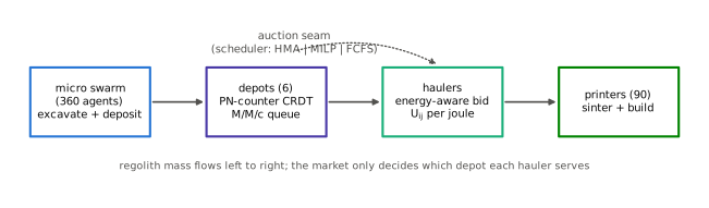
3.1. Conceptual overview. The system has two scales and one seam between them. Micro agents excavate regolith and deposit it at depots; macro agents — haulers and printers — clear those depots and turn their contents into structure. The depots are the seam: they buffer mass so that the micro production rate and the macro consumption rate need not match instant by instant, and they expose their inventory as a replicated counter so that a hauler can reason about depot state without a consistent global view. Every allocation decision in the system is the answer to one question — which depot should this hauler serve next? — and the three schedulers we compare differ only in how they answer it. Throughout, we report throughput (kg of regolith printed), mobility energy per kilogram , and idle fraction .
3.2. Energy-aware auctions (the HMA core). Hauler bids on the task of clearing depot with the utility
where is the mass available at depot . The first term is the heart of the mechanism: it is mass recovered per joule spent, so a hauler prefers the depot that yields the most regolith for the least travel, and the market as a whole therefore allocates scarce hauling capacity to the highest-marginal-value depot rather than the nearest or the first to ask. The gate is a sigmoid on state-of-charge that drives a hauler’s bids toward zero as it approaches the critical reserve , so a depleted hauler withdraws from the market instead of stranding itself; it is smooth rather than a hard threshold so that it relaxes cleanly into the MILP comparator’s continuous formulation, and the same specification is used everywhere in this paper (reproduced in Appendix A). The second term prices delay, charging a bid for the time the hauler would spend travelling and then waiting in the depot’s queue.
Bids are cleared by local coordinators at each depot on a fixed ten-second rolling batch auction, which is also the replan cadence granted to the central planner, so the comparison does not turn on one scheduler being allowed to think more often than another. Ties — bids within 1% of one another — are broken by a wear-levelling score (Appendix E). To avoid the message storm of a fully-connected market, auctions are spatially pruned: each depot solicits only the nearest haulers within radius . The mechanism is implemented in gossamer.algorithms.coordination.hma.
3.3. Depot buffers and micro policies. Depots hold regolith between the scales, and the micro swarm maintains their inventory through local density control rather than any central quota. Because a depot may be written by many micro agents concurrently and read by haulers that cannot be assumed to share a consistent view, its inventory is represented as a PN-counter CRDT: increments and decrements commute, so replicas that diverge under partition converge again on merge without a coordinating authority. This is the same design decision as the auction’s — the system must keep working when the agents cannot agree in real time.
3.4. Rate balance. The system is a pipeline, so its throughput is set by its narrowest stage, and its energy cost accumulates across all three:
The experiments in §5 deliberately sweep the middle term: by varying the mass a hauler can carry per trip, we walk from far below the micro production rate to far above it, which is what moves the system between the regimes where scheduling matters and where it does not.
3.5. Queueing analysis, and the regime in which it is valid. Model each depot as an M/M/c queue: haulers serve arrivals from the micro layer at rate (kg/s), each clearing mass at rate (kg/s). Write the offered load and the utilization . When the queue is stable and its mean length is given by the Erlang-C formula,
with the probability an arrival must wait. The buffer’s purpose follows directly: it must absorb plus a margin, since a depot that runs dry starves its printers and a depot that overflows has immobilized regolith that the fleet paid to move.
This apparatus is only defined for , and that condition is doing real work in this paper. As the mean queue diverges; at arrivals outrun service, no steady state exists, and is infinite. A buffer cannot decouple two rates that are not, on average, equal — it can only absorb their variance. We stress this because the contended regime that carries our headline result turns out to sit at (§5.4), where the standard “the buffer decouples the scales” argument does not hold, and where what the market actually does is something else. Earlier drafts of this work asserted the decoupling as a design property; the committed runs instrument , , and per depot and compute the M/M/c prediction alongside the measured wait, which is what allowed us to find that the assertion was false in exactly the regime we cared about.
Little’s Law. Independently of any M/M/c assumption, the identity holds for any stationary queue, and we use it as the measured wait throughout: is derived from the observed mean queue and arrival rate rather than from the model. Where we report a theoretical M/M/c wait, it is labelled as such, and it is reported as undefined when rather than as a plausible finite number.
4. Experimental Setup / Simulation Environment
The result is an algorithmic claim about a scheduling policy, so the environment is a simplified 3-D kinematic abstraction, not a grain-level lunar-surface model: regolith is carried as per-agent inventory, agents advance under velocity-Verlet integration, and all quantities are in raw simulation units (§5). The lunar-ISRU framing is the motivating scenario; the numbers back the coordination policy, not physical hardware.
4.1. Simulation platform. The physics is Leviathan (velocity-Verlet integration, bounded domain, max_speed clamp), executing the Gossamer HMA primitive and orchestrated by Maneuver.Map against a fixed seed tree. The engine’s energy and fault modules are disabled so that the scheduler is the only variable: with the energy module active, agents drain charge as and begin failing within roughly eighty steps, which would confound every throughput comparison with an attrition effect that has nothing to do with allocation.
4.2. Scenario design. Each run holds agents — 360 micro (regolith processing), 30 haulers, and 90 printers — serving 6 depots, for 8,000 steps at s, i.e. 4,000 seconds of simulated operation. Micro agents feed the depots; haulers clear the depots to the printers. The hauler capacity — the mass one hauler can move per trip — is the swept load parameter, and sweeping it is what walks depot utilization and thereby moves the system between the regimes of §5.
A correction to the previous version of this section, which described the wrong fleet. Earlier text stated with 150 haulers. That is the configuration of the uncontended control batch, not of the capacity sweep — and every headline number in this paper comes from the sweep, which runs 30 haulers. The two batches therefore differed in both hauler count and hauler capacity, which means the old “uncontended control” was never a control: it varied two things at once. This revision drops that comparison entirely. The over-provisioned regime is now measured within the sweep’s own fleet (capacity 50, 30 haulers), where it is a genuine one-variable contrast.
4.3. Design points. The results rest on one committed batch: a 20-seed capacity sweep, 3 hauler capacities × 3 schedulers × 20 seeds = 180 cells. The market uses an SOC threshold of throughout.
The seed count is the whole point of this revision. The previous version reported 5 seeds, and at the seed-to-seed spread of printed mass was roughly a third of the mean — so a +29% effect and a null were statistically indistinguishable by construction, whichever one was true. Twenty seeds is what makes the confidence intervals in §5 narrow enough to adjudicate anything, and adjudicating is what they do: they turn one of our headlines into a null and another into a significant loss.
4.4. Baselines. We compare three schedulers that share one physics substrate, one utility specification, and one stepping loop, differing only in how a hauler is matched to a depot. FCFS serves depots in arrival order — the naive baseline. The MILP central planner solves the depot–hauler assignment with OR-Tools under a fixed 0.5 s per-replan time budget, returning the best feasible solution found within that budget; it is the credible centralized comparator, and its behavior under load (§5.5) turns out to be informative in its own right. HMA (ours) is the decentralized energy-aware auction of §3.2. The central planner is genuinely dispatched rather than aliased: the runner refuses to start a milp_ortools cell if OR-Tools is unavailable rather than silently falling back to the auction, which would have made the paper’s central comparison a comparison of the market against itself.
4.5. Metrics, and how we adjudicate them. We report printed mass, mobility energy per kilogram, printer idle fraction, reallocation latency, and the per-depot queueing observables (arrival rate , service rate , wait , queue , utilization ) — all in raw simulation units, as means ± s.d. over 20 seeds.
Each scheduler is compared against the FCFS baseline with a Welch -test and a 95% confidence interval on the difference. Welch rather than Student because the schedulers have no reason to share a variance and — as §5.5 shows — they emphatically do not. We read a null off a confidence interval that straddles zero, never off a -value alone, and we treat a result as a loss only when the whole interval sits on the wrong side of zero. This matters here because the previous version of this paper reported point estimates without intervals, and the point estimate was the thing that was wrong.
4.6. Reproducibility. Batch hma_remeasure-20260712T180940-7d0c8ed3 (180 cells); every cell carries the standard provenance block (Appendix F).
5. Results
The results below are measured from one committed batch on the real (Leviathan-pinned) engine, Gossamer 0.7.0: hma_remeasure — 180 cells, three schedulers × 20 seeds × hauler capacity ∈ 50. Each run is agents (360 micro / 30 haulers / 90 printers, 6 depots), 8,000 steps at s (4,000 s of simulated operation). All quantities are raw simulation units; the physical-unit calibration used elsewhere in this manuscript (kg/h, Wh/kg) is a separate mapping and is not applied here. We lead with the dimensionless cross-scheduler ratios, which need no calibration. Every scheduler shares one utility specification and one physics substrate; only the allocation policy differs (hma decentralized auction, milp_ortools central planner with a 0.5 s per-replan budget, fcfs naive baseline). Comparisons are Welch tests with 95% CIs on the difference against FCFS (§4.5).
5.1. The market wins under scarcity, ties in the middle, and loses when over-provisioned. The ranking of the three schedulers is not fixed across the capacity sweep — but it does not vary in the way we previously reported. It varies monotonically against the market:
Table 1. Printed mass by hauler capacity and scheduler (mean ± s.d. over 20 seeds), each scheduler against the FCFS baseline.
| Cap | Scheduler | Printed mass (kg) | vs FCFS | 95% CI of difference | Verdict | |
|---|---|---|---|---|---|---|
| 10 | FCFS | 14,486 ± 1,833 | — | (baseline) | — | — |
| 10 | MILP central | 18,910 ± 5,275 | +30.5% | [+1,843, +7,004] kg | 3.54 | win |
| 10 | HMA | 19,359 ± 5,975 | +33.6% | [+1,979, +7,767] kg | 3.49 | win |
| 25 | FCFS | 35,775 ± 4,540 | — | (baseline) | — | — |
| 25 | MILP central | 35,479 ± 9,149 | −0.8% | [−4,976, +4,383] kg | −0.13 | null |
| 25 | HMA | 33,178 ± 9,883 | −7.3% | [−7,590, +2,395] kg | −1.07 | null |
| 50 | FCFS | 61,597 ± 4,332 | — | (baseline) | — | — |
| 50 | MILP central | 53,338 ± 6,155 | −13.4% | [−11,679, −4,840] kg | −4.91 | loss |
| 50 | HMA | 54,719 ± 6,377 | −11.2% | [−10,384, −3,373] kg | −3.99 | loss |
Three statements, and the second and third are the ones that bite.
The market is real, and it is narrow. Under genuine scarcity a decentralized auction decisively beats the naive scheduler: +33.6%, , with a confidence interval comfortably clear of zero. The central planner tracks it (+30.5%). This is the result we would defend, and it is arguably the more useful one, because scarcity is not an edge case for a fleet operator — it is what operating near your capital’s limit looks like.
A tie is not the boundary; a loss is. One rung up, at capacity 25, the effect vanishes into a null. One rung further, when haulers are over-provisioned, both sophisticated schedulers are significantly worse than first-come-first-serve (−11.2% and −13.4%, –5). This is not the graceful convergence the previous version described. When there is no scarcity to allocate, the market’s marginal-value routing sends haulers past nearer depots to reach higher-value ones, and the extra travel buys nothing: throughput falls and mobility energy per kilogram rises by 13.6% (§5.3). The machinery is not merely unnecessary outside its regime — it is actively costly.
Therefore every claim this mechanism makes carries a capacity precondition, not a caveat. “The market improves throughput” is false as stated. “The market improves throughput when hauling capacity is scarce, and reduces it when it is not” is what the data support, and the difference between those two sentences is the difference between a useful result and a misleading one.
5.2. There is no uncontended control, and the previous one was confounded. The earlier version of this paper anchored the “schedulers converge when supply is ample” claim to a capacity-500 batch. That batch runs a different fleet — 150 haulers against the sweep’s 30 (§4.2) — so it varied hauler count and hauler capacity simultaneously and could not isolate either. We have dropped it. The over-provisioned regime is now measured inside the sweep’s own fleet at capacity 50, which is a genuine one-variable contrast, and it does not show convergence: it shows the market losing.
5.3. Mobility energy: the advantage does not survive, and outside scarcity the sign flips. The published claim was a 20–29% reduction in energy per kilogram. At 20 seeds it is weaker everywhere and reverses outside the scarce regime.
Table 2. Mobility energy per kilogram (lower is better; mean ± s.d. over 20 seeds).
| Cap | Scheduler | E/kg | vs FCFS | 95% CI of difference | Verdict | |
|---|---|---|---|---|---|---|
| 10 | FCFS | 109.2 ± 12.8 | — | (baseline) | — | — |
| 10 | MILP central | 91.1 ± 35.2 | −16.6% | [−35, −1] | −2.16 | win |
| 10 | HMA | 92.4 ± 44.2 | −15.4% | [−38, +4] | −1.64 | null |
| 25 | FCFS | 44.5 ± 7.5 | — | (baseline) | — | — |
| 25 | MILP central | 47.2 ± 13.3 | +6.1% | [−4, +10] | 0.79 | null |
| 25 | HMA | 51.2 ± 14.9 | +15.0% | [−1, +14] | 1.78 | null (sign flipped) |
| 50 | FCFS | 25.5 ± 1.9 | — | (baseline) | — | — |
| 50 | MILP central | 29.6 ± 3.5 | +16.4% | [+2, +6] | 4.65 | loss |
| 50 | HMA | 28.9 ± 3.7 | +13.6% | [+2, +5] | 3.74 | loss |
Even where the market is at its best — capacity 10, where it wins decisively on throughput — its energy advantage is a null: the point estimate is favourable (−15.4%) but the interval straddles zero. Only the central planner achieves a clean energy win there. At capacity 25 the published −22% becomes +15.0%, a sign flip. At capacity 50 it is a significant loss. We therefore withdraw the energy-per-kilogram claim entirely — §5.7 already argued it was immaterial at system level, and it now turns out not to be a measured effect either.
5.4. The depots are saturated everywhere — and the drainage mechanism works only where the market wins. The M/M/c instrumentation says, unambiguously and at , that the depots are not operating as buffers. All 180 cells report (–6 at capacity 10, –3 at 25, and still –1.7 at the “over-provisioned” capacity 50). A queue at has no steady state: arrivals outrun service, the theoretical wait diverges, and the finite we measure is a transient backlog, not a stationary wait. This is the one major claim of the previous version that the re-measurement strengthened rather than refuted, and it kills the buffer-decoupling story (H2) outright, in every regime, including the one we called over-provisioned.
What the market does instead is drain that backlog faster — and it does so exactly where, and only where, it wins throughput. At capacity 10 HMA holds a shorter depot queue ( vs FCFS’s kg, −4.9%, ) and a correspondingly shorter wait ( vs s, −4.8%, ) at an identical arrival rate ( kg/s in every arm — is set by the micro layer and no scheduler touches it). Little’s Law (, [5]) makes those the same statement. At capacity 25 both differences are nulls. At capacity 50 they invert: HMA holds a queue 27% longer than FCFS’s and a wait 27% longer.
That co-occurrence is the most useful thing in this paper. The mechanism (faster backlog drainage) and the outcome (higher throughput) appear together under scarcity and disappear together outside it — which is what a real mechanism does, and what a spurious one does not.
5.5. The robustness argument is refuted — by our own data, in the opposite direction. The previous version of this paper claimed the market “degrades gracefully” where the budgeted planner “degrades erratically,” and offered that as the sharper operational case for decentralization. It was an artifact of five seeds. At twenty:
Table 3. Seed-to-seed standard deviation as a multiple of FCFS’s, printed mass and energy per kg. Higher is worse.
| Cap | HMA (throughput) | HMA (energy/kg) | MILP (throughput) |
|---|---|---|---|
| 10 | 3.3× | 3.4× | 2.9× |
| 25 | 2.2× | 2.0× | 2.0× |
| 50 | 1.5× | 1.9× | 1.4× |
HMA is the least consistent scheduler at every capacity, on every metric. At the scarce operating point its throughput s.d. (5,975 kg) exceeds even the central planner’s (5,275 kg) — the exact inverse of the published comparison, which reported HMA at ±1,876 against MILP’s ±6,998 on five seeds. Those two numbers were a small-sample illusion.
The honest reading is that the market buys its scarcity win by increasing variance: it explores allocations, and exploration has a spread. That may still be the right trade — a scheduler that is 34% better on average and noisier is a good deal if you can absorb a bad week — but it must be argued as a risk-adjusted trade, not as robustness. A “graceful degradation” framing is not available from this data, and we withdraw it.
Printer idle fraction, finally, is 0.452 in all nine arms, identical to three decimals: the scheduler does not move it at all. The idle-time half of hypothesis H1 is a flat null, and we say so.
5.6. Figures.
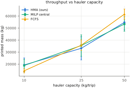
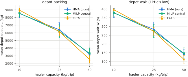
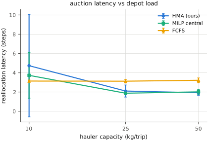
All three figures are drawn from the 20-seed batch by a committed generator that declares, per figure, the batch and the metric it derives from — so a figure cannot silently drift from the data behind it. Figure 3 replaces the fleet state-of-charge panel promised in earlier drafts. State-of-charge is not instrumented in the committed runs — it enters the bid through the SOC gate of §3.2 but is never recorded as a time series — so no such figure can be drawn from this data, and we decline to draw one from anything else. The depot-queue panel is in any case the load-bearing evidence for §5.4.
5.7 Whole-system energy context — a projection, not a measurement
This subsection is an un-calibrated order-of-magnitude projection and must not be cited as a result. It exists to answer one question — would the scheduler’s energy advantage matter at the system level even if it were real? — and the answer is no. Since §5.3 now shows that it is not real (a null under scarcity, a significant loss when over-provisioned), this subsection is doubly moot, and we retain it only to close the question.
The simulation reports mobility energy in raw engine units; converting to Wh/kg requires a sim→physical calibration we have not performed. Sintering energy is worse: the literature spans more than an order of magnitude. A thermodynamic floor for heating regolith to sintering temperature (~1375 K) is a few MJ/kg [10], and we take 2.4 MJ/kg = 667 Wh/kg as that idealized floor; but measured microwave sintering of regolith simulant reports on the order of 69 MJ/kg once process inefficiency is counted [9] — roughly thirty times larger.
Take the mobility term at its most generous: suppose the market really did deliver the ~15% relative reduction its point estimate suggests under scarcity. Against a sintering floor of 667 Wh/kg — the assumption most favourable to our own result — mobility is under a tenth of whole-system energy, so a 15% relative saving on it is worth roughly 1% of system energy. Against a realistic sintering figure [9], some thirty times larger, it disappears entirely. So the energy argument was never load-bearing even in the world where it was true, and it is not that world.
We therefore do not claim energy per kilogram as a contribution, and the reader should not infer one from the tables in §5.3. The load-bearing claim of this paper is now a single one: the scarcity-conditional throughput win (§5.1), with the backlog-drainage mechanism (§5.4) as its evidence, and the over-provisioned loss (§5.1) as its precondition.
6. Discussion
6.1. What the results mean. Our first hypothesis (H1) — that energy-aware auctions raise throughput and reduce idle time relative to FCFS — is partially supported, and the qualification is the finding. The throughput half holds under scarcity (+33.6%, ) and reverses when haulers are over-provisioned (−11.2%, ). The idle-time half is a flat null: printer idle is 0.452 in every arm at every capacity. And the energy half, which we advanced as a co-headline, does not survive at all (§5.3).
The shape of the error is worth naming, because it is more instructive than the correction. We reported a market that helped in the middle and was harmlessly redundant at the extremes. What we actually have is a market that helps under scarcity and actively hurts when capacity is abundant. Those two pictures agree about the regime where the market is useful and disagree completely about the cost of deploying it outside that regime — and it is the second thing, not the first, that a fleet operator needs to know, because it is the one that can lose them throughput they already had.
Our second hypothesis (H2) — that depot buffers decouple the macro and micro rates — is refuted outright, and more comprehensively than we previously admitted. The mechanism requires a stable queue (); all 180 cells run at , including the arm we called over-provisioned. There is no regime in this study where the buffer-decoupling argument applies. What the market does instead is drain the saturated backlog faster — and, tellingly, it does that only at the capacity where it also wins throughput (§5.4). The mechanism and the outcome appear and disappear together, which is what distinguishes a real effect from a coincidence, and it is the strongest evidence in the paper.
6.2. Relation to prior work. That market mechanisms beat first-come allocation under resource constraints is not new; it is the central finding of the multi-robot task-allocation literature [3, 4]. Dias et al. [4] warn that a market optimizes a sum of local utilities and can therefore be led astray by a badly-chosen utility — and our over-provisioned regime is a clean instance of exactly that failure. Our per-joule utility tells a hauler to prefer the depot with the best mass-per-joule ratio. Under scarcity that is the right instruction. When haulers are abundant, it sends them past nearer depots toward marginally richer ones, and the fleet pays for the travel without gaining anything, because there was no allocation problem to solve. The market is not broken in that regime; it is faithfully optimizing an objective that has stopped corresponding to throughput.
Our contribution is therefore narrower and, we think, more useful than “markets beat greedy”: we place the market against a credible central optimum under a realistic per-replan budget, and we report the boundary of its usefulness rather than only its best operating point.
6.3. Implications. For a fleet designer the practical reading is about sizing, and it now carries a warning it did not before. The first design question is whether the fleet will operate under hauling scarcity. If it will not, do not deploy the market: at capacity 50 it costs 11% of throughput against a scheduler you can implement in an afternoon. If it will, the market is worth a great deal — but budget for the variance (§5.5), because the win comes with a seed-to-seed spread 1.5–3.4× the baseline’s, and a scheduler with a better mean and a wider distribution is a risk-adjusted choice rather than an unambiguous one.
We no longer argue for decentralization on robustness grounds. That case rested on the market degrading more gracefully than the budgeted planner, and at 20 seeds the market is the less consistent of the two. What survives is a narrower and more honest argument: under scarcity, a decentralized auction matches a central planner’s allocation quality without the planner’s solve-time budget, and beats a naive baseline by a third.
6.4. On the tooling. The separation of concerns across the stack — physics in Leviathan, coordination primitives in Gossamer, orchestration in Maneuver.Map — is what made the three-scheduler comparison trustworthy, because all three schedulers provably step through identical physics and differ only at the allocation seam.
It is also, twice now, what caught our own errors. The queueing instrumentation lived in the coordination library and, once actually called, refuted the buffer hypothesis this paper was built to advance. And the figure generator declares the batch behind every figure, which is how a headline pinned to a superseded model version became visible rather than persistent. We record this because the correction in Appendix F was not found by a reviewer; it was found by the instrumentation, and that is the argument for building the instrumentation.
7. Limitations and Future Work
7.1. Limitations. The most important gap is that adversarial robustness is not modeled. The auction as specified is open to Sybil bidders, to falsified depot-inventory reports, and to coordinated denial-of-delivery; a lunar construction fleet is a high-value target, and a market that assumes honest bids is a market with an attack surface. We flag this as the single most important next axis rather than a footnote.
The wear model is a tiebreaker, not a system: cumulative service time stands in for wear and is consulted only when competing bids fall within 1% of one another. Wear-aware bidding, in which wear enters the utility function directly and the fleet trades throughput against its own longevity, is future work and would likely change the allocation qualitatively rather than marginally.
Several physical models are deliberately coarse. The sintering thermal model is single-zone, using a midrange 2.4 MJ/kg constant where real lunar sinter has chemistry-dependent regimes (sulfur-bearing versus anhydrous regolith). There is no solar-storm shadowing or radiation degradation, terrain heterogeneity is limited to the heightmap-and-density-layer abstraction of Appendix B, and communications are idealized beyond what the Leviathan comms model captures — in particular we do not model spoofed control packets, which is the same gap as the adversarial one seen from the network side.
Finally, and most consequentially for how these numbers should be read: the regolith transport is kinematic, not physical (Appendix B), and the absolute throughput figures are therefore properties of this abstraction rather than predictions about hardware. The cross-scheduler ratios, which share every one of those abstractions, are what we ask the reader to rely on.
7.2. Future work. The clear next steps are Sybil-resistant auction protocols (bid commitments, reputation, threshold cryptography), integrating wear into the bid utility rather than the tiebreak, heterogeneous micro roles, hardware-in-the-loop printing tests, and learned depot sizing as a function of the solar duty cycle. The adversarial axis is the one we consider load-bearing for any real deployment.
8. Conclusion
Energy-aware market scheduling raises throughput by a third over a naive baseline — under scarcity, and only under scarcity. When hauling capacity is abundant the same mechanism costs 11% of throughput and 14% more mobility energy per kilogram, both significant at 20 seeds. That precondition is not a footnote to the result; on any fleet that is not capacity-constrained, it is the result.
Three of our claims did not survive their own instrumentation, and we have said so rather than quietly restating them. The depot buffer does not decouple the macro and micro rates: every cell we measured runs saturated, so the mechanism has no regime in which it applies. Mobility energy is not a contribution: it is a null where the market is strongest and a loss where it is weakest. And the market is not the more predictable scheduler — it is the least consistent of the three, at every capacity, on every metric, which is the exact opposite of what we previously claimed and removes robustness as a fallback argument for decentralization.
What remains, and what we would defend, is a single sharp result: under genuine hauling scarcity a decentralized auction matches a budgeted central planner and beats first-come-first-serve by 33.6%, by draining a saturated depot backlog faster at matched arrival rate — with the mechanism and the outcome appearing together, and vanishing together, at exactly the same point on the capacity axis. That is a narrower paper than the one we set out to write. It is also, we think, a more useful one, because it tells a fleet operator not only when to reach for a market but when reaching for one will cost them.
Resilience under agent failure is not demonstrated here: the fault module is disabled in every run so that the scheduler is the only variable, and the adversarial and fault-tolerance axes (§7) remain the most important open work.
Data and Code Availability
Every result in §5 derives from one immutable experiment batch: hma_remeasure-20260712T180940-7d0c8ed3 (180 cells — 3 hauler capacities × 3 schedulers × 20 seeds). Each cell is a directory containing an experiment.json carrying its full configuration, provenance block, and metrics. The figures in §5 are generated directly from that batch by a committed script that declares, per figure, the batch and metric it derives from, so a figure cannot silently drift from the data behind it; the reduction (Welch tests, CIs on the difference) is likewise a committed script rather than a spreadsheet.
The two batches behind the superseded version of this paper — hma_paper-20260710T214442-b5d0aae7 (15 cells) and hma_load-20260710T214629-1f5bed81 (75 cells) — remain published as the provenance of the withdrawn claims. They are not reproducible on any wheel we can still build (Appendix F), and no current figure or table is drawn from them. The per-result mapping is maintained in the reproducibility runbook.
References
[1] R. G. Smith, “The Contract Net Protocol: High-Level Communication and Control in a Distributed Problem Solver,” IEEE Transactions on Computers, vol. C-29, no. 12, pp. 1104–1113, 1980. doi:10.1109/TC.1980.1675516
[2] L. E. Parker, “ALLIANCE: An Architecture for Fault-Tolerant Multirobot Cooperation,” IEEE Transactions on Robotics and Automation, vol. 14, no. 2, pp. 220–240, 1998.
[3] B. P. Gerkey and M. J. Matarić, “A Formal Analysis and Taxonomy of Task Allocation in Multi-Robot Systems,” International Journal of Robotics Research, vol. 23, no. 9, pp. 939–954, 2004. doi:10.1177/0278364904045564
[4] M. B. Dias, R. Zlot, N. Kalra, and A. Stentz, “Market-Based Multirobot Coordination: A Survey and Analysis,” Proceedings of the IEEE, vol. 94, no. 7, pp. 1257–1270, 2006. doi:10.1109/JPROC.2006.876939
[5] J. D. C. Little, “A Proof for the Queuing Formula: ,” Operations Research, vol. 9, no. 3, pp. 383–387, 1961.
[6] D. Gross, J. F. Shortle, J. M. Thompson, and C. M. Harris, Fundamentals of Queueing Theory, 4th ed., Wiley, 2008. (M/M/c, Erlang-C, and the stability condition.)
[7] M. Shapiro, N. Preguiça, C. Baquero, and M. Zawirski, “Conflict-Free Replicated Data Types,” Stabilization, Safety, and Security of Distributed Systems (SSS), pp. 386–400, 2011.
[8] “Sintering of Lunar Regolith: A Review,” Acta Astronautica, 2025. doi:10.1016/j.actaastro.2025.02.031
[9] “Sintering of Lunar Regolith Simulants Using a Domestic Microwave: A Rapid and Energy-Efficient Strategy for Construction Material Fabrication,” Journal of the European Ceramic Society, 2024. (Reports ≈69 MJ/kg measured process energy — the figure that bounds our §5.7 projection from above.)
[10] M. Z. Naser and A. I. Chehab, “Energy Requirements of a Thermally Processed ISRU Radiation Shield for a Lunar Habitat,” Advances in Space Research, vol. 66, no. 5, 2020. doi:10.1016/j.asr.2020.03.011
Appendix / Supplementary Material
Appendix A: The Energy-Aware Bid Utility Function (canonical form)
This appendix reproduces the canonical bid utility from §3.2; the two are identical.
Default coefficients (used unless explicitly varied): , s⁻¹, , (30% SOC).
Appendix B: Regolith Handling (Abstraction)
The committed runs represent regolith transport kinematically, matching the algorithmic scope of the claim: micro agents accrue inventory at a per-agent rate and deposit it at depots; haulers carry depot inventory to printers as point masses under the capacity constraint. No grain-level, voxel, or rigid-body dust model is used — the abstraction is deliberate, and the coordination result does not depend on surface physics.
Appendix C: Simulation Parameters
Committed configuration: 360 micro / 30 hauler / 90 printer agents () across 6 depots, 8,000 steps at s, HMA SOC threshold , MILP budget 0.5 s per replan. The swept parameter is hauler capacity , each at 3 schedulers × 20 seeds = 180 cells.
(Previous versions of this appendix listed 150 haulers and . That is the fleet of the superseded capacity-500 control batch, not of the sweep that produced every reported number — see §4.2.)
Appendix D: Committed Parameters
The table below is the committed configuration. No component ablation was run. Earlier drafts of this appendix announced three ablations — auctions without the SOC penalty, depots without buffering, and a central planner on a fixed cadence — that were never executed and for which no batch exists; the claim has been removed rather than reworded. Isolating which component drives the throughput gain versus the energy gain remains open, and the load sweep of §5 is a regime study, not an ablation.
| Parameter | Value | Notes |
|---|---|---|
| Micro Agents | ||
| Count () | 360 | Regolith processing |
| Macro Fleet | ||
| Haulers | 30 | Clear depots to printers |
| Printers | 90 | Consume depot inventory |
| Depots | 6 | M/M/c service points |
| Hauler capacity | swept | The load parameter; sets depot utilization |
| Seeds | 20 per cell | 3 caps × 3 schedulers × 20 = 180 cells |
| Market | ||
| SOC threshold | 0.30 | Energy-aware bid gate |
| MILP budget | 0.5 s | Per replan (central comparator) |
Appendix E: Wear Model
Cumulative service-time wear . Used as a tiebreaker when competing bids are within 1% of each other. Future-work bidding-side integration would use but is not enabled in the §5 results.
Appendix F: Reproducibility, and the correction this revision makes
The §5 results are committed. Every table and figure comes from one batch — hma_remeasure-20260712T180940-7d0c8ed3 (180 cells) — run on the real engine at Gossamer 0.7.0 (NumPy 2.2.6): three schedulers (hma / milp_ortools / fcfs) × 3 hauler capacities 50 × 20 seeds, , 8,000 steps, s. The OR-Tools MILP comparator is genuinely dispatched under a 0.5 s per-replan budget — the runner refuses to start a milp_ortools cell if OR-Tools is unavailable rather than silently falling back to the auction, which would have made this paper’s central comparison a comparison of the market against itself. See Reproducibility and Data Availability. Symbol conventions follow the unified table in ICCD Appendix F.
What this revision changes, and why. The previously published version of this paper reported +29% printed mass at hauler capacity 25. That number does not reproduce, and it is now known to have been wrong in two independent ways. We set both out, because the second is the more important and the less obvious.
First, the model changed. A refactor of the HMA world model (0.6.0 → 0.7.0) re-implemented the micro→depot assignment as a vectorized reduction over squared distances where it had been a scan over hypot distances. The two are mathematically equivalent orderings but not bit-identical, and the system amplifies the difference: one flipped depot assignment changes which hauler serves which queue, and over 8,000 steps that cascades. The runs are individually deterministic — physically identical replicas return byte-identical output — so this was a genuine change in the modelled dynamics, not simulator noise. The published batch is reproducible only on the 0.6.0 wheel, and nothing can restore it.
Second, and this is the real lesson: five seeds could never have adjudicated the claim in the first place. At the seed-to-seed spread of printed mass was about a third of the mean. A +29% effect and a null were therefore statistically indistinguishable by construction — the experiment as designed could not have told them apart, whichever was true. The refactor is what made us look; it is not what made the number wrong. The number was never supported. Had the model never changed, we would have gone on quoting a headline our own error bars could not sustain.
The re-measurement at settles it, and the verdict is not a small correction:
| Claim (as published) | At |
|---|---|
| +29% printed mass at capacity 25 | null (−7.3%, CI [−7,590, +2,395] kg, ) |
| +35% at capacity 10 | reproduces (+33.6%, CI [+1,979, +7,767] kg, ) |
| “schedulers converge” when over-provisioned | false — HMA is −11.2% (), a significant loss |
| −22% mobility energy per kg at capacity 25 | null, and the sign flips (+15.0%) |
| HMA is the more predictable scheduler (§5.5) | false — HMA’s s.d. is 1.5–3.4× FCFS’s at every capacity |
Only one of the five survived — and it is at the capacity below the one the paper built its headline on. The corrected claim is narrower, and stated as a precondition rather than a caveat: the market’s advantage is real, large, and confined to scarcity, and outside scarcity it is a measurable liability.
We also record a plain description error, since the previous text misdescribed the very runs it reported: §4.2 and Appendix C gave the fleet as with 150 haulers. That is the configuration of the capacity-500 control batch. The sweep behind every headline number ran 30 haulers, — so the old “uncontended control” differed from the sweep in two variables at once and was never a valid control. It has been withdrawn, and the over-provisioned regime is now measured inside the sweep’s own fleet.
Finally, the general lesson we would ask a reader to take from this appendix, because it cost us a headline: a refactor that moves a published number is a detectable event, and a sample too small to support that number is not. The first failure announced itself. The second was silent for months, and would have stayed silent indefinitely, because a plausible number does not raise an exception. The seed count, not the refactor, is the thing that should have been checked first.